Dynamic HTML
A user doesn't need any app installed to interact with sliders in your notebook
Please read the manual carefully.
This is a dynamic version of the Static HTML exporter, designed to recreate the full interactivity of normal notebooks.

Use Cases
- All use cases from Static HTML
- Demonstration projects
- Live animations of physical processes
- Interactive presentations / lecture notes
Demonstration 🚀
See what can be exported
How It Works
To make the system more general and support features like ManipulatePlot, Manipulate, combinations of InputRange, InputButton, Offload, FrontSubmit, EmitSound, and many more are abstracted from their controlling elements. The system purely analyzes events and symbol mutations.
Your dynamic system must follow a call and response architecture. That means it must generate events (via user interaction or code) and produce a response (e.g., symbol mutation or FrontSubmit).
TL;DR: We record calculated data for all possible combinations of input elements and store them in a large table. The missing values are interpolated using IDW method. See the How to Use section.
Details
Analysis
To analyze the bindings between input elements, symbols, and commands executed by the Wolfram Kernel, we inject a spy into the evaluation kernel by modifying DownValues of WLJS I/O symbols. This captures symbol mutations triggered by external events and submitted commands like FrontSubmit or EmitSound. For instance, PlotlyAnimate also uses FrontSubmit and can be tracked.
After capturing all data, it's forwarded to samplers or virtual state machines.
Processing
We use different processing techniques based on the use case, selected automatically. These are known as Black Boxes or virtual machines.
Similar to airplane black boxes that record all data for post-crash analysis.
There are three types of virtual machines (automatically chosen) with fun names:
State Machine
This tracks system state based on input element combinations. It samples all possible states and dispatches the corresponding symbol mutations.
In the runtime it attempts to interpolate the missing values using:
- Inverse Distance Weighting (IDW) in continuous feature space.
- Categorical conditioning: It filters/selects neighbors based on matching categorical values, so interpolation is performed within semantically similar groups.
- If the output is not a number of numeric tensor, it attempts to interpolate strings if they contain some number-like features and composes them back after.
Pavlov Machine
Like Pavlov's Dog, it doesn't track state but records event → FrontSubmit pairs.
Animation Machine
Detects series of symbol mutations from the same event, typically used for animations (e.g., via AnimationFrameListener). It tracks only abstract frame numbers.
How to Use
Please follow the steps below:
Prepare the Notebook
Connect to the Wolfram Kernel and evaluate your dynamics. Minimize the number of input elements and their states. For example, avoid 3 sliders (InputRange) with 100 steps each. For ManipulatePlot, explicitly set step values. Limit the number and complexity of dynamic symbols.
If you're recording an animation with AnimationFrameListener, start it right before the next step. Note: SetInterval effects are not captured.
Example using a single slider:
ManipulatePlot[{
  Sum[(Sin[2π(2j - 1) x])/(2j - 1), {j, 1, n}],
  Sum[(Cos[2π(2j - 1) x])/(2j - 1), {j, 1, n}]
} // Re, {x, -1, 1}, {n, 1, 10, 1}]
Try to use a reasonable number of sliders and steps per slider. For example, 3 sliders with 100 steps each would result in 1,000,000 possible states to sample. If you skip too many steps, WLJS will attempt to interpolate between them in your HTML using the IDW (Inverse Distance Weighting) method.
Sniffing Phase
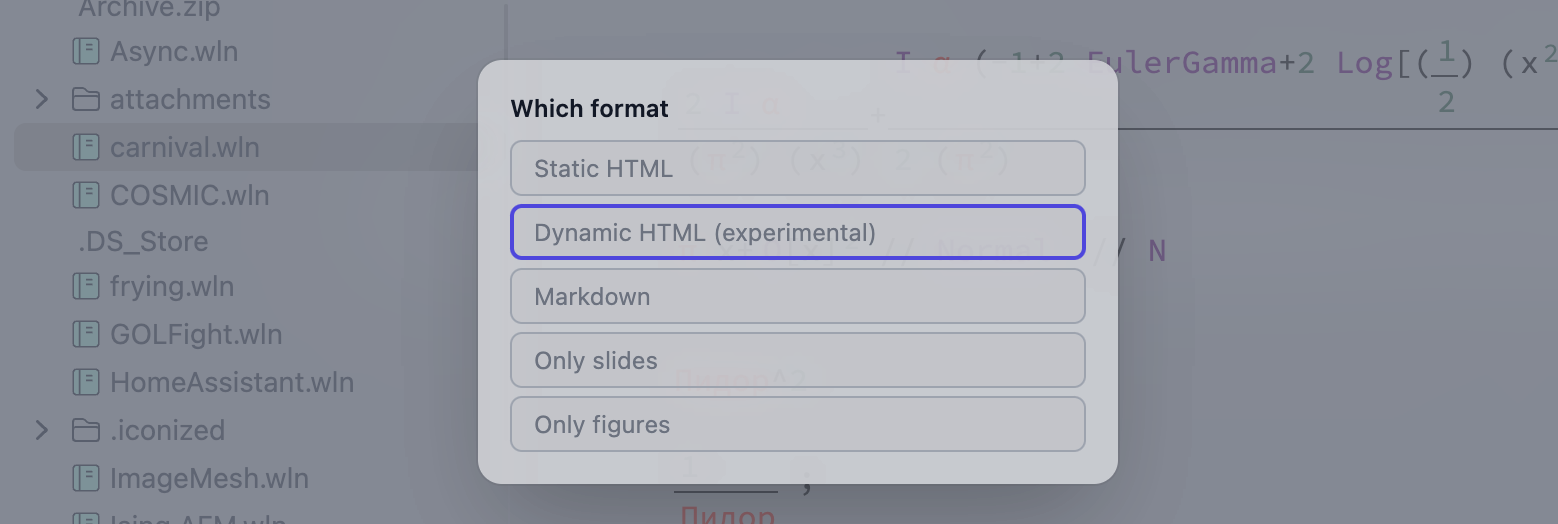
Click Share → Dynamic Notebook to begin recording. A widget will appear in the top-right corner.
If you're recording an animation, evaluate the cell and wait for your desired number of frames, then click Continue in the widget.
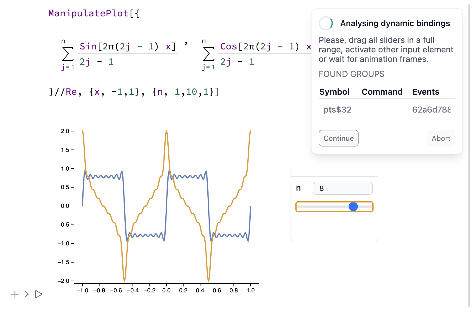
Move each slider across its full range. This is necessary, as the sampling phase will only use values seen during sniffing.
For multiple inputs (2–3 sliders), move each fully once. Cross-combinations are not needed—they will be resampled recursively automatically.
Sampling Phase (State Machine)
Now the system automatically samples all input combinations. This may take time, depending on state count and symbol complexity.
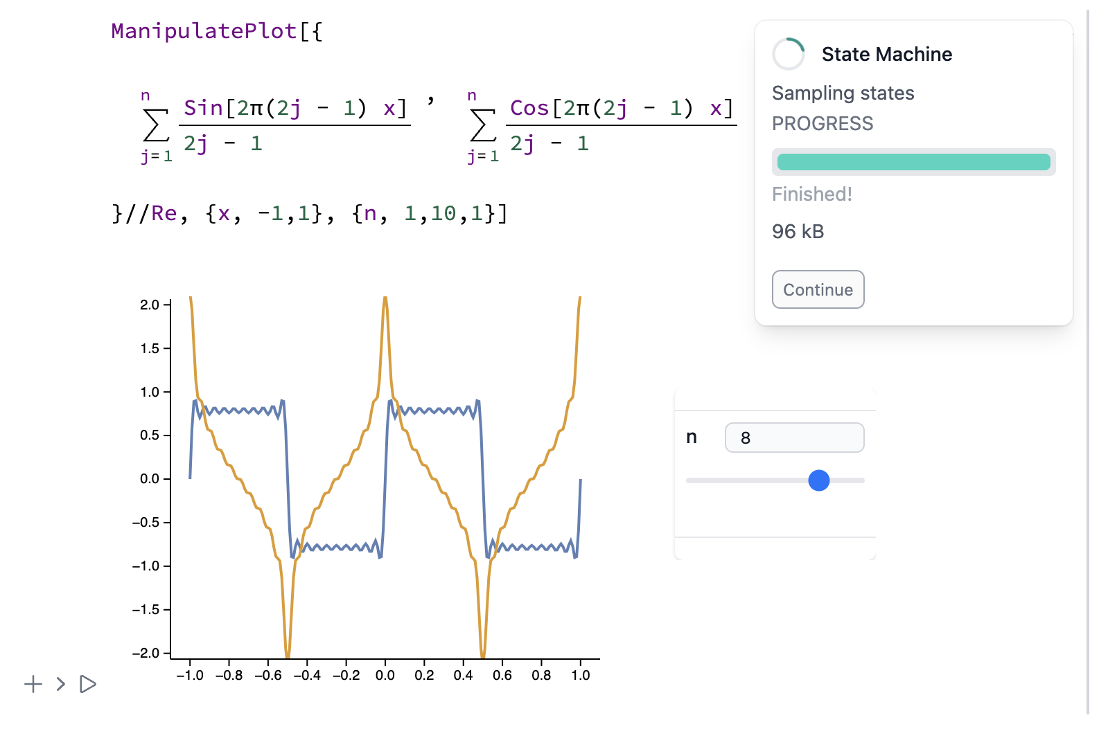
This is the final stage. Afterward, the notebook is exported with the collected data to your drive. Click Continue.
Result
File sizes typically range from 7–20 MB, or 3–15 MB with CDN settings (see Static HTML). The example above is just 165 kB uncompressed and 50 kB compressed.
The result is a fully interactive widget, working offline without an internet connection or the Wolfram Kernel ✨
What Else Can Be Exported?
Here's a list of supported exports:
State Machine
Manipulate[Series[Sin[x], {x, 0, n}], {n, 1, 10, 1}]
ManipulatePlot[f[w x], {x, -10, 10}, {w, 0, 10}, {f, {Sinc, Sin}}]
Video Tutorial
Slider and selection
Many sliders
Or custom dynamics:
radius = 1.0;
Graphics[{Hue[radius // Offload], Disk[{0, 0}, radius // Offload]}, ImageSize -> Small]

EventHandler[InputRange[0, 1, 0.1], (radius = #)&]
Or continuous features on 2D canvas
Video Tutorial
Or continuous Manipulate
Manipulate[Column[{
  Style[StringTemplate["`` m/s"][x], Blue],
  Table["🚗", {i, Floor[x/25]}]//Row
}], {x,10,100}, ContinuousAction->True] // Quiet
Video Tutorial
The missing values will be interpolated using our own method: Categorical-Aware Inverse Distance Weighted Interpolation (IDW) with support for structured output decomposition and recomposition.
That also means: more features you sample -- more accurate result will be reproduced for the continuously changing data.
Pavlov Machine
EventHandler[InputButton[], (Sound[SoundNote["C5"]] // EmitSound)&]
Even Plotly:
p = Plotly[{<|
  "values" -> {19, 26, 10},
  "labels" -> {"Residential", "Non-Residential", "Utility"},
  "type" -> "pie"
|>}]

EventHandler[InputRange[0, 100, 10], PlotlyAnimate[p,
  <|"data" -> {<|"values" -> {19, 26, #}|>},
    "traces" -> {0}
  |>, <||>]&
]
- Click Share
- Drag sliders / click buttons
- Press continue
Animation Machine
Example: balls falling down a staircase
Video Tutorial
An example with Animate
Animate[Row[{Sin[x], "==", Series[Sin[x], {x,0,n}], Invisible[1/2]}], {n, 1, 10, 1}, AnimationRate->3]
AnimatePlot does not need to be exported using dynamic HTML. It works with basic static as well.
Video Tutorial
Other Examples
Check out some interactive examples from our blog and demo projects: